Varianzanalyse und Kovarianzanalyse für unabhängige Stichproben
Erforderliche Pakete laden
library(afex)   # ANOVA
library(car)    # Robuste ANOVA
library(emmeans)# Zellmittelwerte berechnen
Datensatz einlesen und Variablen spezifizieren
# Datensatz einlesen
Programm <- rep(c("Programm 1", "Programm 2", "Programm 3"), each=6, times=2)
Instruktion <- rep(c("Instruktion 1", "Instruktion 2"), c(18,18))
Intelligenz <- c(5,6,6,4,3,5,5,7,7,9,6,6,8,7,5,4,7,6,7,6,4,4,6,5,6,8,7,5,5,8,5,6,5,5,4,5)
Testleistung <- c(13,17,18,10,9,12,10,14,17,19,11,14,21,19,13,13,16,15,20,16,14,12,19,15,17,22,19,13,12,20, 14,25,22,19,15,18)
data <- data.frame(Programm, Instruktion, Intelligenz, Testleistung)

# Variablen spezifizieren
between <- c("Programm", "Instruktion")   # Namen der Faktoren mit unabhängigen Stichproben eingeben
AV <- "Testleistung"                      # Name der abhängigen Variable eingeben
KV <- c("Intelligenz")                    # Namen der Kovariablen eingeben. Falls keine Kovariablen: KV <- NULL
Deskriptive Statistik, Signifikanztest, Effektstärke und Teststärke
# Listwise Deletion (Zeilen mit Missings in den berücksichtigten Variablen eliminieren)
data2 <- na.omit(data[,c(AV, KV, between)])
# Der Datensatz muss eine Spalte "Block" mit den Probanden-IDs enthalten.
data2$Block <- as.factor(1:nrow(data2))
# Betweenfaktoren als Faktoren definieren
if (length(between) > 1){
data2[,between] <- lapply(data2[,between], as.factor)
} else {
data2[,between] <- as.factor(data2[,between])
}

# Deskriptive Statistik
if (is.null(KV)) {
Kennwerte <- function(x) c(n=length(x), mean=mean(x), sd=sd(x), se=sd(x)/sqrt(length(x)))
Formel <- as.formula(paste(".~", paste(between, collapse="+")))
deskriptive.statistik <- aggregate(Formel, data2[,c(between, AV)], Kennwerte)
} else {
Kennwerte <- function(x) c(mean=mean(x), sd=sd(x), se=sd(x)/sqrt(length(x)))
Formel <- as.formula(paste(".~", paste(between, collapse="+")))
tab <- aggregate(Formel, data2[,c(between,  AV, KV)], Kennwerte)
n <- aggregate(Formel, data2[,c(between, AV)], length)
deskriptive.statistik <- data.frame(tab,n=n[,ncol(n)])
data2[,KV] <- scale(data2[,KV],center=TRUE, scale=FALSE)  # Mittelwertzentrierung der KV für ANCOVA
}

# Signifikanztest mit Quadratsummenzerlegung nach Modell III
library(afex)
TAB <- aov_ez(id="Block", dv=AV, data=data2, between=between, covariate=KV, factorize=FALSE, return="Anova")

# Partielles Eta-Quadrat und Power
Effekte <- length(TAB[,1])-2
Power <- vector(length=Effekte)
eta.sq <- vector(length=Effekte)
df2<- TAB["Residuals",2]
for (i in 1:Effekte){
df1<- TAB[i+1,2]
eta.sq[i] <- TAB[i+1,1]/(TAB[i+1,1]+TAB["Residuals",1])
ncp<- TAB[i+1,3]*df1    # Analog SPSS: ncp=f^2*df2=(F*df1/df2)*df2; (G*Power: ncp=f^2*N)
Fk<- qf(1-0.05,df1,df2)
Power[i]<- 1-pf(Fk, df1=df1, df2=df2, ncp=ncp)}
# Tabelle mit EtaQuadrat und Power
eta.sq.Power <- data.frame(eta.sq, Power)
rownames(eta.sq.Power) <- rownames(TAB)[-c(1, nrow(TAB))]

# Berechnung der Least–Square-Mittelwerte bzw. Rand-Mittelwerte
library(emmeans)
Faktoren <- as.formula(paste("~", paste(between, collapse="*")))
if (is.null(KV)) {
  model <- as.formula(paste(AV, "~", paste(between, collapse="*")))
  TAB2 <- lm(model, data2)
  ls.means <- lsmeans(TAB2, Faktoren)
} else {
  model <- as.formula(paste(AV, "~", paste(between, collapse="*"), "+", paste(KV, collapse="+")))
  TAB2 <- lm(model, data2)
  ls.means <- lsmeans(TAB2, Faktoren)
}

list("Deskriptive Statistik" = deskriptive.statistik, ANOVA=TAB, eta.sq.Power=eta.sq.Power, "Geschätzte Randmittelwerte"=ls.means)
## $`Deskriptive Statistik`
## Programm Instruktion Testleistung.mean Testleistung.sd Testleistung.se
## 1 Programm 1 Instruktion 1 13.166667 3.656045 1.492574
## 2 Programm 2 Instruktion 1 14.166667 3.430258 1.400397
## 3 Programm 3 Instruktion 1 16.166667 3.250641 1.327069
## 4 Programm 1 Instruktion 2 16.000000 3.033150 1.238278
## 5 Programm 2 Instruktion 2 17.166667 3.970726 1.621042
## 6 Programm 3 Instruktion 2 18.833333 4.167333 1.701307
## Intelligenz.mean Intelligenz.sd Intelligenz.se n
## 1 4.8333333 1.1690452 0.4772607 6
## 2 6.6666667 1.3662601 0.5577734 6
## 3 6.1666667 1.4719601 0.6009252 6
## 4 5.3333333 1.2110601 0.4944132 6
## 5 6.5000000 1.3784049 0.5627314 6
## 6 5.0000000 0.6324555 0.2581989 6
##
## $ANOVA
## Anova Table (Type III tests)
##
## Response: dv
## Sum Sq Df F value Pr(>F)
## (Intercept) 9120.2 1 2864.0317 < 2.2e-16 ***
## Programm 101.9 2 16.0009 2.076e-05 ***
## Instruktion 111.2 1 34.9169 2.045e-06 ***
## Intelligenz 297.8 1 93.5240 1.403e-10 ***
## Programm:Instruktion 22.9 2 3.6033 0.04003 *
## Residuals 92.3 29
## ---
## Signif. codes: 0 '***' 0.001 '**' 0.01 '*' 0.05 '.' 0.1 ' ' 1
##
## $eta.sq.Power
## eta.sq Power
## Programm 0.5246046 0.9988454
## Instruktion 0.5462861 0.9999097
## Intelligenz 0.7633117 1.0000000
## Programm:Instruktion 0.1990415 0.6203478
##
## $`Geschätzte Randmittelwerte`
## Programm Instruktion lsmean SE df lower.CL upper.CL
## Programm 1 Instruktion 1 15.5 0.768 29 13.9 17.1
## Programm 2 Instruktion 1 11.8 0.768 29 10.3 13.4
## Programm 3 Instruktion 1 15.1 0.737 29 13.6 16.6
## Programm 1 Instruktion 2 17.1 0.737 29 15.6 18.6
## Programm 2 Instruktion 2 15.3 0.755 29 13.7 16.8
## Programm 3 Instruktion 2 20.7 0.755 29 19.2 22.3
##
## Confidence level used: 0.95Im Fall einer Kovarianzanalyse überprüfen, ob Interaktionen zwischen den Faktoren und den Kovariablen bestehen
if (!is.null(KV)) {
  modell <- as.formula(paste0(AV, "~", paste(between, collapse="*"), "* (", paste(KV, collapse="+"), ")"))
  anova(lm(modell, data2))
}
## Analysis of Variance Table
##
## Response: Testleistung
## Df Sum Sq Mean Sq F value Pr(>F)
## Programm 2 52.167 26.083 8.3964 0.00172 **
## Instruktion 1 72.250 72.250 23.2577 6.520e-05 ***
## Intelligenz 1 275.037 275.037 88.5361 1.592e-09 ***
## Programm:Instruktion 2 22.949 11.474 3.6937 0.03995 *
## Programm:Intelligenz 2 0.140 0.070 0.0226 0.97767
## Instruktion:Intelligenz 1 2.692 2.692 0.8667 0.36115
## Programm:Instruktion:Intelligenz 2 14.959 7.480 2.4078 0.11143
## Residuals 24 74.556 3.106
## ---
## Signif. codes: 0 '***' 0.001 '**' 0.01 '*' 0.05 '.' 0.1 ' ' 1Diagnostikplots
if (is.null(KV)) {
  modell <- as.formula(paste0(AV, "~", paste(between, collapse="*")))
} else {
modell <- as.formula(paste0(AV, "~", paste(between, collapse="*"), "+", KV))}
m <- lm(modell, data2)
par(mfrow=c(2,2), bty="n")
plot(m)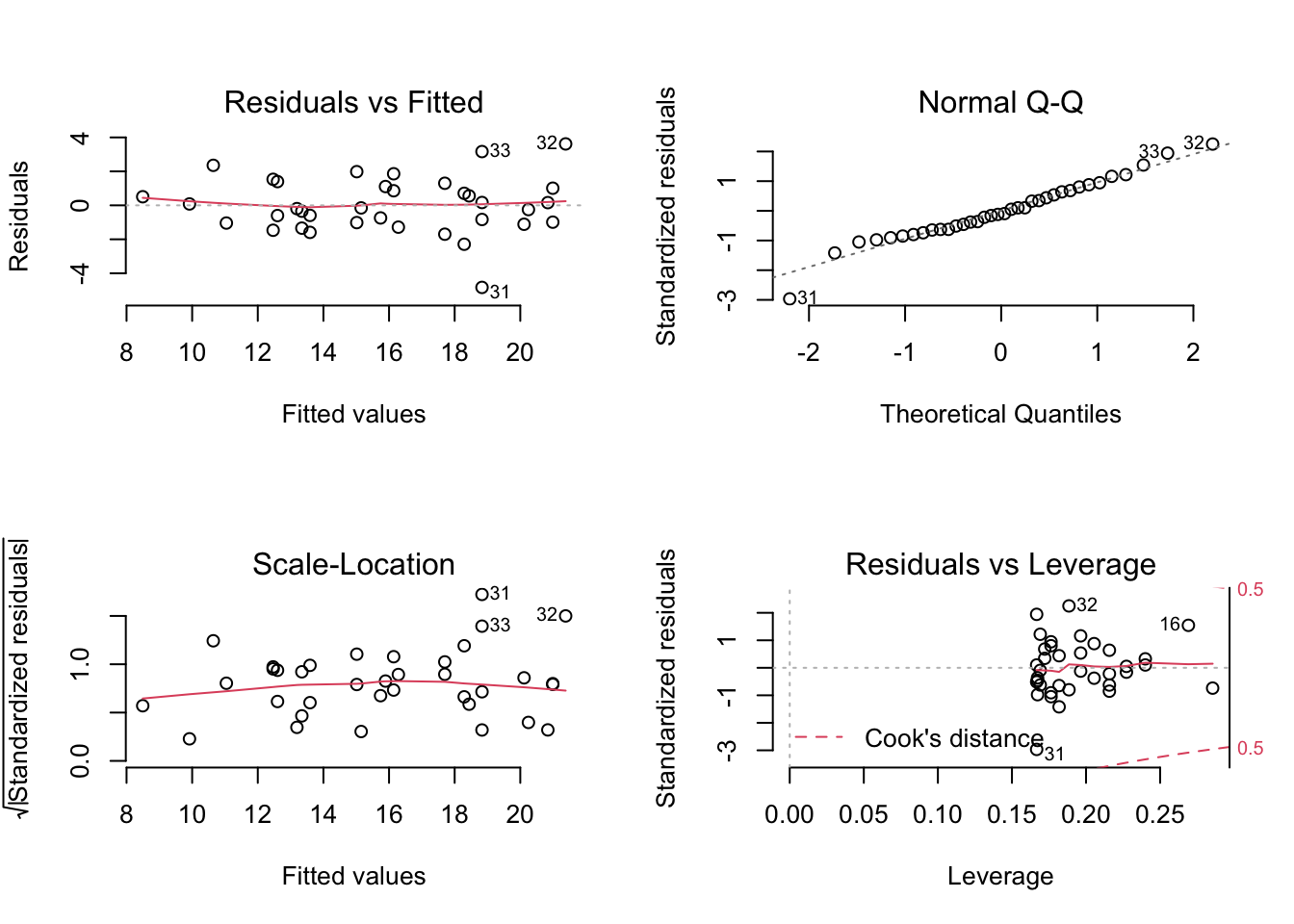
Robuste ANOVA: Korrektur der Heteroskedastizität
library(car)
if (is.null(KV)) {
  modell <- as.formula(paste0(AV, "~", paste(between, collapse="*")))
} else {
modell <- as.formula(paste0(AV, "~", paste(between, collapse="*"), "+", KV))}
options(contrasts=c("contr.sum","contr.poly"))
m <- lm(modell, data=data2)
Anova(m, type="III", white.adjust=TRUE)
## Coefficient covariances computed by hccm()## Analysis of Deviance Table (Type III tests)
##
## Response: Testleistung
## Df F Pr(>F)
## (Intercept) 1 2352.6722 < 2.2e-16 ***
## Programm 2 13.4564 7.343e-05 ***
## Instruktion 1 27.8324 1.179e-05 ***
## Intelligenz 1 104.4251 4.029e-11 ***
## Programm:Instruktion 2 2.5806 0.09301 .
## Residuals 29
## ---
## Signif. codes: 0 '***' 0.001 '**' 0.01 '*' 0.05 '.' 0.1 ' ' 1Geplante Vergleiche
Die unten verwendete Funktion contrast() berechnet die Prüfgrösse t wie folgt:
# Means <- summary(M)$lsmean; Contrast <- unlist(C); t <- sum(Contrast*Means)/sqrt(QSe/(n*dfe)*sum(Contrast^2))
# Means = Geschätzte Randmittelwerte, Contrast = Kontraskoefizienten
# QSe = Fehlerquadratsumme, dfe= Fehlerfreiheitsgrade, n = Zellgrösse
# QSe und dfe können aus der ANOVA-Tabelle abgelesen werden.
Beispiel 1: Haupteffektkontrast Programm (3 vs. 1 und 2)
Die Abfolge der Kontrastkoeffizienten muss derjenigen der Stufen entsprechen.
C <- list(c(-1,-1,2))           # Programm (3 vs. 1 und 2)
M <- lsmeans(TAB2, ~Programm)   # Least–Square-Mittelwerte
## NOTE: Results may be misleading due to involvement in interactionscontrast(M, C)## contrast estimate SE df t.ratio p.value
## c(-1, -1, 2) 6.02 1.27 29 4.749 0.0001
##
## Results are averaged over the levels of: InstruktionBeispiel 2: Interaktionskontrast Programm (3 vs. 1 und 2) * Instruktion (1 vs. 2)
Programm <- c(-1,-1,2)                            # Programm (3 vs. 1 und 2)
Instruktion <- c(-1,1)                            # Instruktion (1 vs. 2)
C <- list(as.numeric(Programm %o% Instruktion))   # Programm (3 vs. 1 und 2) * Instruktion (1 vs. 2)
M <- lsmeans(TAB2, ~Programm+Instruktion)         # Least–Square-Mittelwerte
contrast(M, C)
## contrast estimate SE df t.ratio p.value
## c(1, 1, -2, -1, -1, 2) 6.3 2.62 29 2.404 0.0228Post-hoc-Vergleiche nach Tukey
M <- lsmeans(TAB2, ~Programm+Instruktion)
tukey <- contrast(M, method="pairwise"); tukey
## contrast estimate SE df t.ratio
## Programm 1 Instruktion 1 - Programm 2 Instruktion 1 3.673 1.14 29 3.228
## Programm 1 Instruktion 1 - Programm 3 Instruktion 1 0.399 1.09 29 0.366
## Programm 1 Instruktion 1 - Programm 1 Instruktion 2 -1.559 1.04 29 -1.501
## Programm 1 Instruktion 1 - Programm 2 Instruktion 2 0.248 1.12 29 0.222
## Programm 1 Instruktion 1 - Programm 3 Instruktion 2 -5.242 1.03 29 -5.083
## Programm 2 Instruktion 1 - Programm 3 Instruktion 1 -3.275 1.04 29 -3.153
## Programm 2 Instruktion 1 - Programm 1 Instruktion 2 -5.232 1.09 29 -4.806
## Programm 2 Instruktion 1 - Programm 2 Instruktion 2 -3.425 1.03 29 -3.321
## Programm 2 Instruktion 1 - Programm 3 Instruktion 2 -8.915 1.12 29 -7.960
## Programm 3 Instruktion 1 - Programm 1 Instruktion 2 -1.958 1.05 29 -1.858
## Programm 3 Instruktion 1 - Programm 2 Instruktion 2 -0.150 1.03 29 -0.145
## Programm 3 Instruktion 1 - Programm 3 Instruktion 2 -5.641 1.08 29 -5.246
## Programm 1 Instruktion 2 - Programm 2 Instruktion 2 1.807 1.08 29 1.681
## Programm 1 Instruktion 2 - Programm 3 Instruktion 2 -3.683 1.03 29 -3.562
## Programm 2 Instruktion 2 - Programm 3 Instruktion 2 -5.490 1.10 29 -4.975
## p.value
## 0.0331
## 0.9990
## 0.6665
## 0.9999
## 0.0003
## 0.0394
## 0.0006
## 0.0266
## <.0001
## 0.4466
## 1.0000
## 0.0002
## 0.5546
## 0.0148
## 0.0004
##
## P value adjustment: tukey method for comparing a family of 6 estimatesplot(tukey)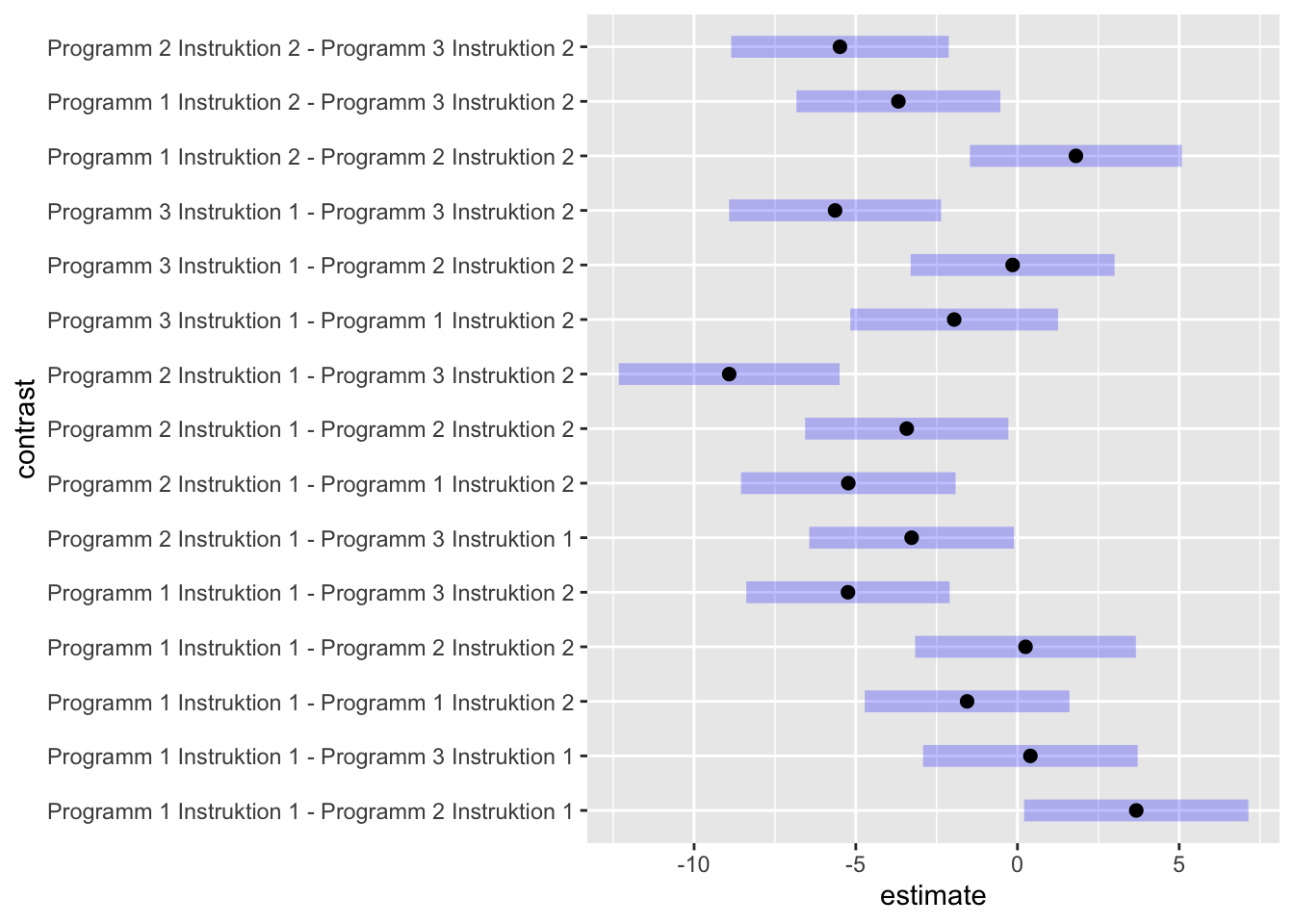
Grafiken
Hinweis: Interaktionsplot mit den geschätzten Randmittelwerten
Bei Kovarianzanalysen kann der Interaktionsplot der Mittelwerte anders aussehen als der Interaktionsplot der adjustierten Mittelwerte.
# Faktornamen spezifizieren
Faktor1 <- "Programm"     # Name des ersten Faktors eingeben (Abszisse)
Faktor2 <- "Instruktion"  # Name des zweiten Faktors eingeben (Farbe)
AV <- "Testleistung"      # Name der abhängigen Variable eingeben
data.aggr <- summary(ls.means)  # Datensatz mit Mittelwerten und KI generieren

# "Liniendiagramm für Mittelwerte" aufrufen
# Den Code für die "Schwarzweissversion" oder die "Farbige Version" des entsprechenden Designs laufen lassen.
# Es werden die Mittelwerte mit 95%-Konfidenzintervallen dargestellt.