Hauptkomponenten- und Hauptachsenanalyse
Skript mit Erklärung der Verfahren und Vorgehensweisen anhand von Beispielen.
Erforderliche Pakete laden
library(psych) # Hauptkomponenten- und HauptachsenanalyseDatensatz einlesen und Variablen spezifizieren
# Die Daten können entweder als Rohdaten oder als Korrelationsmatrix eingegeben werden.
# Korrelationsmatrizen müssen folgende Struktur haben:
# Erste Zeile: Variablenbezeichnungen
# Zweite Zeile: Stichprobenumfang
# Dritte Zeile: Mittelwerte
# Vierte Zeile: Standardabweichungen
# Korrelationsmatrix: Die obere Dreiecksmatrix darf Nullen enthalten.
# Alternativen zur Pearson'schen Korrelation finden Sie mit ?tetrachoric.
data <- read.table(file="https://mmi.psycho.unibas.ch/r-toolbox/data/Faktorenanalyse/Faktorenanalyse3.txt", header=TRUE)

# Variablen spezifizieren
# Falls die Korrelationsmatrix gegeben ist, alle Variablen berücksichtigen.
Variablen <- 1:6
Daten <- "Matrix"     # Für Korrelationsmatrix: Daten <- "Matrix". Sonst Daten <- "Rohdaten"
Analyse <- "pa"       # Hauptkomponentenanalyse "pc", Hauptachsenanalyse "pa"
Rotation <- "varimax" # Rotationstyp "none", "varimax", oder "oblimin"
Faktoren <- 2         # Anzahl zu extrahierender Faktoren (Komponenten)
covar <- FALSE # Faktorisierung der Korrelationsmatirx. Faktorisierung der Kovarianzmatrix: covar <- TRUE
Hauptkomponenten- oder Hauptachsenanalyse
# Datensatz data2 für die Analyse
library(psych)
if (Daten=="Rohdaten") {
data2 <- as.matrix(na.omit(data[, Variablen, drop=FALSE]))
} else {
data <- as.matrix(data)
N <- as.numeric(data[1,1])  # Stichprobengroesse einlesen
matr <- data[4:nrow(data),] # Dreiecksmatrix einlesen
# Dreiecksmatrix in symmetrische Matrix verwandeln
matr[upper.tri(matr)] <- t(matr)[upper.tri(matr)]
SD <- as.matrix(data[3,])   # Standardabweichungen einlesen
matr <- SD%*%t(SD)*matr # Kovarianzmatrix berechnen
data2 <- matr
}

# Kaiser, Meyer, Olkin Measure of Sampling Adequacy
if (Daten=="Rohdaten") {
  kmo <- KMO(data2); n.obs <- NA
} else {
  kmo <- KMO(cov2cor(data2)); n.obs=N
}

# Hauptkomponenten- oder Hauptachsenanalyse
if (Analyse=="pc"){
  m <- principal(data2, nfactors=Faktoren, rotate=Rotation, covar=covar, n.obs=n.obs)
  Faktorwerte <- m$scores
} else {
  m <- fa(data2, nfactors=Faktoren, rotate=Rotation, fm="pa", covar=covar, n.obs=n.obs)
  Faktorwerte <- factor.scores(data2, m)$scores
}

if (Rotation=="oblimin") list("Anti-image correlation"=kmo$Image, KMO=kmo, Analyse=m, Strukturmatrix=m$Structure) else list("Anti-image correlation"=kmo$Image, KMO=kmo, Analyse=m)
## $`Anti-image correlation`
## Mathematik Physik Chemie Deutsch Geschichte
## Mathematik 1.00000000 -0.44623745 -0.30876656 -0.01370159 0.03203551
## Physik -0.44623745 1.00000000 -0.20253593 -0.05115466 -0.02581167
## Chemie -0.30876656 -0.20253593 1.00000000 -0.04789996 -0.03147128
## Deutsch -0.01370159 -0.05115466 -0.04789996 1.00000000 -0.31716767
## Geschichte 0.03203551 -0.02581167 -0.03147128 -0.31716767 1.00000000
## Französisch -0.06098249 -0.09908774 -0.08632636 -0.41594627 -0.45154812
## Französisch
## Mathematik -0.06098249
## Physik -0.09908774
## Chemie -0.08632636
## Deutsch -0.41594627
## Geschichte -0.45154812
## Französisch 1.00000000
##
## $KMO
## Kaiser-Meyer-Olkin factor adequacy
## Call: KMO(r = cov2cor(data2))
## Overall MSA = 0.81
## MSA for each item =
## Mathematik Physik Chemie Deutsch Geschichte Französisch
## 0.77 0.81 0.87 0.83 0.81 0.80
##
## $Analyse
## Factor Analysis using method = pa
## Call: fa(r = data2, nfactors = Faktoren, n.obs = n.obs, rotate = Rotation,
## covar = covar, fm = "pa")
## Standardized loadings (pattern matrix) based upon correlation matrix
## PA1 PA2 h2 u2 com
## Mathematik 0.15 0.81 0.67 0.33 1.1
## Physik 0.25 0.72 0.58 0.42 1.2
## Chemie 0.26 0.62 0.45 0.55 1.3
## Deutsch 0.78 0.25 0.68 0.32 1.2
## Geschichte 0.81 0.20 0.70 0.30 1.1
## Französisch 0.83 0.31 0.79 0.21 1.3
##
## PA1 PA2
## SS loadings 2.11 1.76
## Proportion Var 0.35 0.29
## Cumulative Var 0.35 0.64
## Proportion Explained 0.55 0.45
## Cumulative Proportion 0.55 1.00
##
## Mean item complexity = 1.2
## Test of the hypothesis that 2 factors are sufficient.
##
## The degrees of freedom for the null model are 15 and the objective function was 2.84 with Chi Square of 556.63
## The degrees of freedom for the model are 4 and the objective function was 0
##
## The root mean square of the residuals (RMSR) is 0
## The df corrected root mean square of the residuals is 0
##
## The harmonic number of observations is 200 with the empirical chi square 0.01 with prob < 1
## The total number of observations was 200 with Likelihood Chi Square = 0.01 with prob < 1
##
## Tucker Lewis Index of factoring reliability = 1.028
## RMSEA index = 0 and the 90 % confidence intervals are 0 0
## BIC = -21.18
## Fit based upon off diagonal values = 1
## Measures of factor score adequacy
## PA1 PA2
## Correlation of (regression) scores with factors 0.92 0.88
## Multiple R square of scores with factors 0.85 0.77
## Minimum correlation of possible factor scores 0.69 0.54Grafiken
# Scree Plot: Nur wenn Korrelationsmatrix faktorisiert wird
if (covar==TRUE){
  print("Screeplot nicht geeignet, wenn die Kovarianzmatrix faktoriseirt wird.")
} else {
  par(bty="n")
  if (Daten=="Matrix") {
    fa.parallel(cov2cor(data2), n.obs=N)
  } else {
    fa.parallel(data2, n.obs=NULL)
  }
}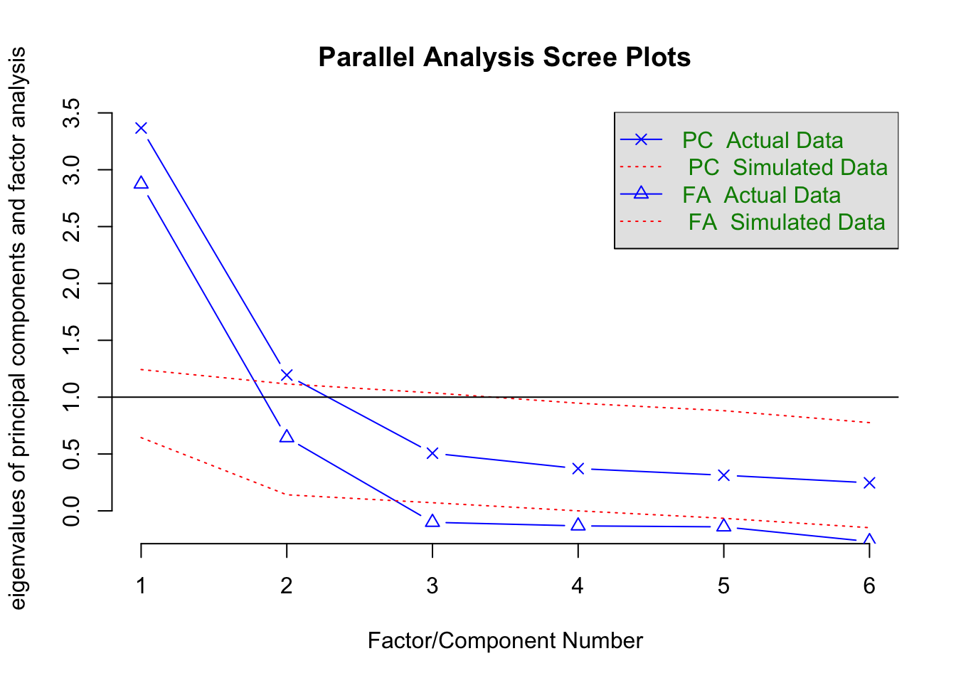
## Parallel analysis suggests that the number of factors = 2 and the number of components = 2# Faktorladungsplot
if (Faktoren>1){
if (Analyse=="pa") m <- fa(data2, nfactors=Faktoren, rotate=Rotation, fm="pa", n.obs=N, covar=covar)
plot(m, xlim=c(-1,1), ylim=c(-1,1), title="Factor Pattern")}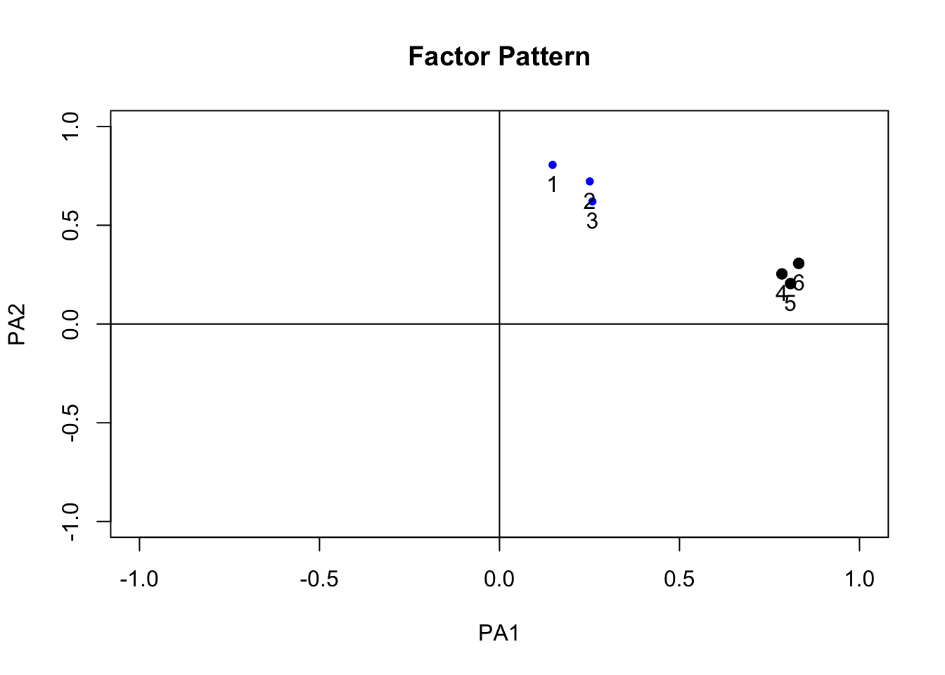
Komponenten resp. Faktoren dem Datensatz hinzufügen
Falls die Rohdaten analysiert wurden, enthält die Variable ‘Faktorwerte’ die Faktorwerte.
# dat <- matrix(nrow=nrow(data), ncol=ncol(Faktorwerte))
# dat[rownames(data) %in% rownames(Faktorwerte),] <- Faktorwerte; colnames(dat) <- colnames(Faktorwerte)
# data <- data.frame(data, dat)